A fundamental quantity for a detector is the noise. The noise, which is usually an additive term, gives a limit to the sensitivity of detector since is impossible or, anyway, very difficult to extract the information from a signal where the informative component has the same or a lower strength than the noise. In the following will be described the behavior of the sensors in absence of any stimuli.
Fixed pattern noise FPN
Even if a matrix of pixels is in dark condition, the pixels are not at the same level. Due to the inevitable differences of a pixel to any other in the matrix, caused by unavoidable non-uniformity in the realization processes, each pixel has a different level in dark.
The fixed pattern noise FPN represents the response of the pixels matrix in case of dark or with a uniform illumination. Strictly speaking, the FPN includes two different components: the dark signal non-uniformity DSNU, that is the response in dark condition, and the photo response non-uniformity PRNU, that represents the different manner with which the pixels react to a uniform irradiation. However, as first approximation, we have assumed that PRNU is negligible and in the following with the term FPN we only refer to the DSNU.
The dark signal non-uniformity represents the offset (often called pedestal) to subtract to all the frames in order to retrieve the signal produced by the radiation. This operation is always performed when we are interested to detect the incident radiation. During our experiments, in fact, the sensors are always shielded by the ambient light and, in order to evaluate the signal produced by the ionizing particles, before each sets of measurements, the FPN is evaluated, stored in the DAQ system and used to calculate the differences unless the sensor does not perform this operation automatically.
In Figure 1 the FPN of one pixel matrix was evaluated collecting 500 consecutive frames and making their average. is shown a representation of this elaboration for the pixels.
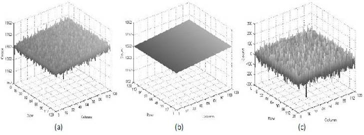
Fig 1 Response of pixel matrix in dark condition (a), with its linear regression to a plane (b) and the relative residues (c).
As can be seen there is a component of the signal that rises linearly with the column number: using a multiple regression algorithm can be extracted the plane shown in Figure 1(b). Subtracting this plane to the measured FPN the values are brought back all around zero (Figure 1c). The equation of plane is:
Y= rαr + cαc + k
where r is the row number and c is the column, αr and αc are the inclination of the plane respectively along columns and along rows and k is a constant term.
Subtracting the interpolating plane the two components discussed above are cancelled and the resulting distribution is centered on zero. In Figure 2a it is shown the distribution of that residuals for the pixel matrix. The distribution has a Gaussian shape with a standard deviation of few tens of counts. Increasing the integration time the shape starts to be slightly different from the Gaussian, in Figure 2b this behavior is emphasized using a logarithmic scale to show the differences at the left of the Gaussian lobe.
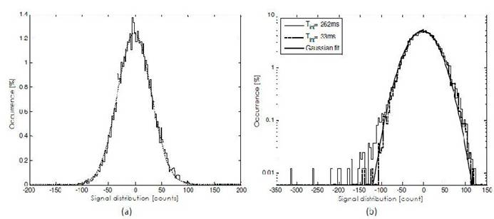
Fig. 2 (a) FPN distribution after subtraction of the interpolating plane of the pxiel matrix (frames collected with 33ms of integration time), and (b) the comparison between this last one and with the same distribution calculated at 262ms of integration time.
Increasing the integration time the pixels voltage must decrease because of the dark current, but the pixels of a matrix don’t behave in a coherent manner: some pixels go towards the discharge faster than others; this means that the dark current is different for each pixel as it should be.
Single Pixel Noise
Each pixel fluctuate around its pedestal from an acquisition to another. The main cause of this fluctuation at the pixel level is the so called kT/C noise but there are some other contributions which increase the level of measured noise as the noise of readout buffer, the quantization noise, external electromagnetic interference, bonding, cables, PCB board, etc.
The Figure 3a is the distribution of the signal measured during 500 consecutive frames on the same pixel: the signal has a Gaussian distribution centered on the pixel’s pedestal. The standard deviation of that distribution differs from pixel to pixel and with the integration time; Figure 3b shows the distribution of that values for the pixel matrix at different integration times. Increasing the integration time the mean noise rise almost linearly in the interval 33ms - 262ms and the spread of the values increase. Due to the asymmetric shape of the distribution the mean value of the measured noise, for a given matrix, differs from the most probable value.
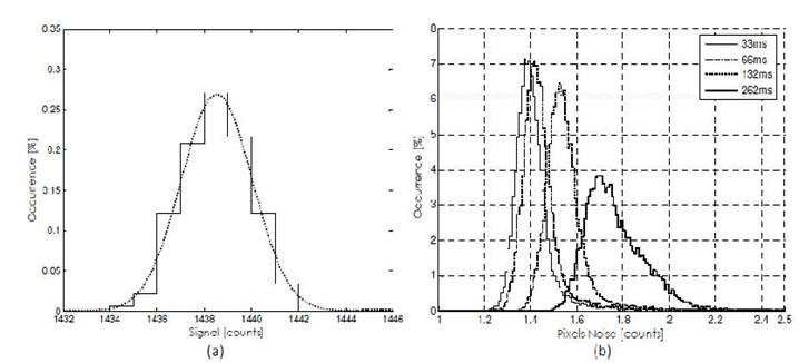
Fig 3 (a) Single pixel noise. (b) Distribution of the single pixel noise for all the pixels of an pixel matrix measured for different integration times.
In Figure 4 are drawn both quantities. As expected the noise is smaller for the matrices with the large photodiode because of its larger capacitance, (indeed the term C occurs at denominator in the expression of kT/C noise power).
Another aspect that can be noted is the dependence of the noise on the integration time: the kT/C noise is, by definition, independent by the time, but this is not true for other contributions such as the leakage current. Indeed, the signal is proportional to the electric charge accumulated into the photodiode and this charge is subjected to a continuous loss due to the leakage current.
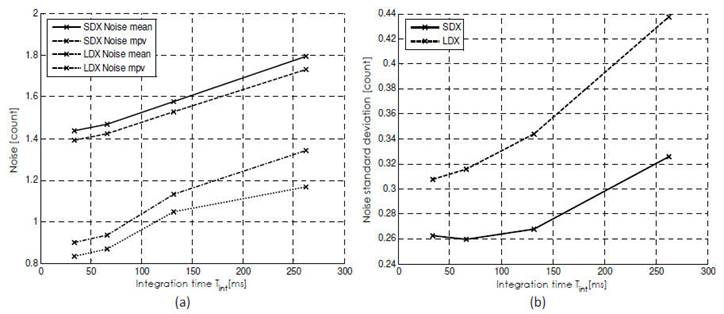
Fig 4 (a) Most probable value of the single pixel noise for four sub-matrix of a pixel matrix chip, for different integration times. (b) Standard deviation of the noise values for all the pixels of two pixel matrices, evaluated at different integration times.
The charge is lose proportional to the time with the relation: Q = I t: if we assume I as a stochastic process with a given variance, Q is a stochastic process in turn with a variance t times higher than the variance of the leakage current.
During acquisition operations, usually, the signal of each pixel, obtained by the difference with the pedestal, is compared with a certain threshold, if the threshold is crossed it is assumed that a particle has crossed the detector and the corresponding frame is collected. Fake crossings, caused by noise, can occur. Usually the threshold must be as lower as possible in order to detect weak signals but the noise puts a lower limit to this parameter. Each frame is composed by Np pixels, assuming the same Gaussian noise for each pixel with a variance σ the probability PFH to have a fake hit is given by:
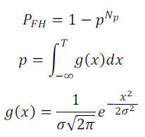
where p is the probability of not crossing the threshold T on a pixel and g(x) is the Gaussian function; using the normalized threshold τ = T/σ the equation becomes:
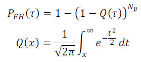
where Q(x) is the so called Q-function.
The PFH can be estimated with the ratio between the number of frames which have crossed a certain threshold on the total frames during an acquisition in dark condition. The measured PFH is reported in Figure 5 with a dotted line. As can be seen the measured quantity differs drastically from the theoretical one.
However, the results of the analysis show that this method is not enough effective to reduce the fake hits. An explanation of this behavior is that there are some pixels (called bad pixel) which have not a Gaussian noise, as shown in Figure 6 where it is reported the evolution of the signal (the graph on the left) and its cumulative distribution (on the right) measured on a particular pixel of the pixel matrix along about 500 consecutive frames.
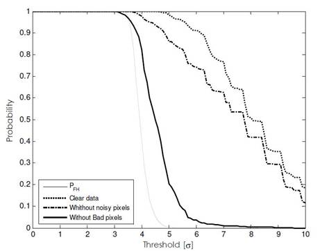
Fig 5. Comparative between the theoretical probability of fake hit (PFH ) in function of the threshold (in units of σ) and the measured one. The bold curves represent the measured probability including into the trigger control: all the pixel (dotted line); only the pixels with noise less than the most probable one (dashed-dotted); excluding the Bad Pixels (solid).
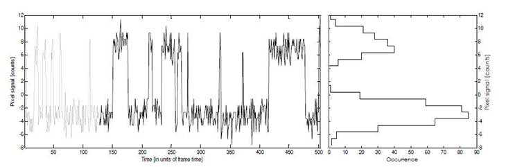
Fig 6. Signal measured on a pixel of the matrix during about 500 consecutive frames (the graph on left) and its cumulative distribution (on right).
If we measure the standard deviation of this pixel, for example, between the 300th and the 400th frame of the figure we will find a value compatible with the most probable noise value of the frame and we would not exclude that pixel from the trigger check, but the leaps clearly visible in the figure could generate fake hits.
References
- D. Passeri et al., Characterization of CMOS Active Pixel Sensors for particle detection: beam test of the four sensors RAPS03 stacked system, Nucl. Instr. and Meth. A 617 (2010) 573–575
- D.Passeri,et al. Tilted CMOS Active Pixel Sensors for Particle Track Reconstruction, IEEE Nucl. Sci. Symp. Conf. Rec. NSS09 (2009) 1678. July 2006.
- L. Servoli et al. . Use of a standard CMOS imager as position detector for charged particles , Nucl. Instr. and Meth. A 215 (2011) 228-231, 10.1016/j.nuclphysbps.2011.04.016
- D. Biagetti et al. Beam test results for the RAPS03 non-epitaxial CMOS active pixel sensor, Nucl. Instr and Meth A 628 (2011) 230–233
Anything missing? Write it here