Spatial Resolution for particle detectors

In order to reconstruct a ionizing particle trajectory, e.g. in High Energy Physics Experiments, it is needed to detect the positions of this particles within the space. The technique used for this purpose consists on the interposition along the trajectory of several sensors planes which are capable to detect the positions where the particles pass through; from the interpolation of all these points can be reconstructed the trajectories followed by the particles. In these environments one of the most important merit figure of the sensors is the spatial resolution, that is the capability to reconstruct the crossing point of the particle.

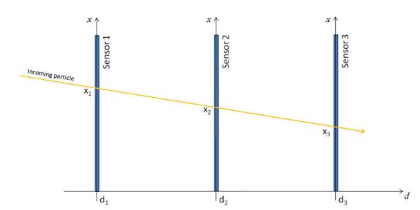
Fig. 1 Illustration of a tracking system with three sensors aligned one in front of each other.

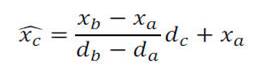
Basically, the evaluation of the spatial resolution of a particle sensor consists on the irradiation of the sensor under test with particles beam at high energy and on the measurement of the differences between the measured impact points with the real ones. It is clear that it is necessary to know the real impact points of the incoming particles, a solution of this problem is to use a known tracking system (usually called telescope) with which it is possible to measure this positions. However a solution that uses only the sensors under test can be used. We can use the same sensors for which we want to measure the resolution to track the particle. The Figure 1 illustrates schematically this system. For simplicity considering a one-dimensional system we can use at least three sensors to detect the coordinate x1, x2 and x3 of the particle trajectory at three different position d1, d2 and d3, from the interpolation of two of these points we can reconstruct the particle path and use them to estimate the position on the third sensor. From simple geometry considerations, if a and b indicate the two sensors used to estimate the position on the third one, that is c, such predicted position will be:

and the difference whit the measured one (in the following called residue also) mathematically is

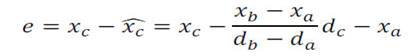
If we assume that the uncertainty in the position measurement has a Gaussian probability density function whit a standard deviation σ, e has a Gaussian probability density function in turn with a deviation of:

  

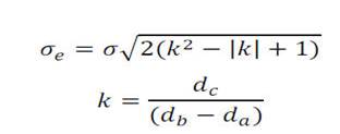
So, from the standard deviation of e and knowing the geometry of the system it is possible to retrieve σwhich is the spatial resolution of the sensors.

The previous example however represents an ideal case; in real cases there are several sources of uncertainty. Each sensor has a non negligible thickness which produces a deflection of the incoming particle due to the phenomenon of multiple scattering. The effect of multiple scattering is to add another aleatory contribution to the coordinates of the measured position. The effect on the residues is to enlarge its distribution; calling σs the deviation introduced by the multiple scattering we can make the approximation:

where σr is the real resolution.

Other sources of uncertainty come from a non perfect alignment of the different elements. Each sensor, as a solid body, has six different degree of freedom, namely three translations and three rotations. The two translations perpendicular to the particles direction adds an offset to the coordinates of the impact point. The effect on the distribution of the residue is only a shift of the Gaussian peak. The translation along the particle direction adds an uncertainty to the coordinate d, however if the distance of a sensor to another is big compared to the position uncertainty this component can be neglected.

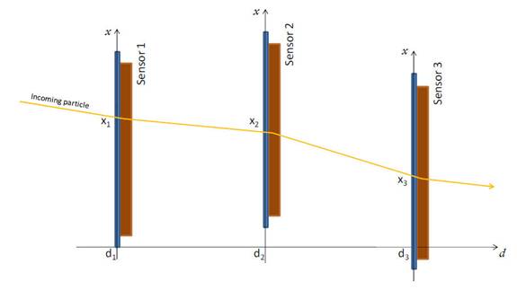
Fig. 2  Effect of the multiple scattering and misalignments in the detection of a particle trajectory.

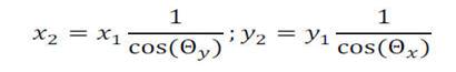
The rotations (Figure 3) are more difficult to compensate. Referring to the Figure 4 a rotation around thex or y axis has the effect shown in Figure 4(a), mathematically:

if the angles are little (few degrees) the correction can be neglected. For the θd tilt the situation is little more complex because each coordinate x or y of a sensor is related to both the coordinates of another sensor (see Figure 4(b)).

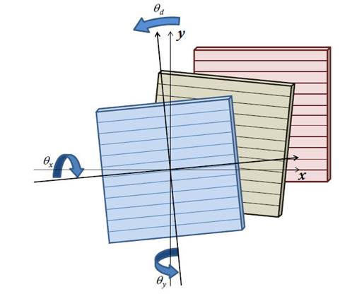
Fig. 3 The three tilt angles among the sensors. 

Mathematically the tilt around the axis parallel to the particles beam direction can be modelled as:

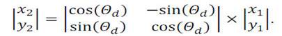
The effect of all the rotation on the residue is to widen its distribution, but from the analysis of the coordinate x2 and y2 detected on a sensor as a function of the coordinate x1 and y2 detected to another sensor the tilt can be estimated and corrected.

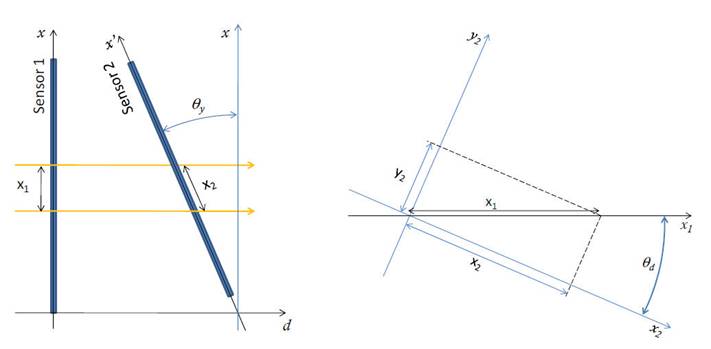
Fig. 4 Effect of a non parallelism among two different sensors.

Summarizing the relation among two different sensors we can consider:

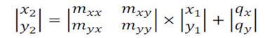
From the measured points, using a multiple linear regression algorithm, it is possible to retrieve the coefficients m and q. 

Another source of uncertainty comes from the algorithm used to define the crossing point of the particles with each single detector. In order to improve the resolution in the position reconstruction, it is possible to exploit the charge sharing effect among adjacent pixels. Usually the barycentre algorithm is used (calledCOG, Center Of Gravity). Mainly due to the finite nature of the detector and the dimensions of the cluster the COG, even if it allows to reach lower resolution limit (i.e. better resolution) than the pixel dimension, it adds a systematic error also.

References

1. D. Passeri et al., Characterization of CMOS Active Pixel Sensors for particle detection: beam test of the four sensors RAPS03 stacked system, Nucl. Instr. and Meth. A 617 (2010) 573–575
2. D.Passeri,et al. Tilted CMOS Active Pixel Sensors for Particle Track Reconstruction, IEEE Nucl. Sci. Symp. Conf. Rec. NSS09 (2009) 1678. July 2006.
3. L. Servoli et al. . Use of a standard CMOS imager as position detector for charged particles ,  Nucl. Instr. and Meth. A 215 (2011) 228-231, 10.1016/j.nuclphysbps.2011.04.016
4. D. Biagetti et al. Beam test results for the RAPS03 non-epitaxial CMOS active pixel sensor, Nucl. Instr and Meth A 628 (2011) 230–233